Load Curves and Load Duration Curves

Topic Name: Load Curves and Load Duration Curves

Introduction

Ever wondered how power companies know just how much electricity we’ll need—and when?

In power systems, effective planning, smooth operation, and cost-effective management all rely on one key factor: understanding how electricity demand changes over time. To analyse and forecast these demand patterns, engineers use two powerful graphical tools—Load Curve and the Load Duration Curve (LDC). These graphical tools help engineers and planners design efficient energy systems, balance supply with demand, and optimise generation capacity.

To illustrate their importance, consider this real-world application:

In rural Kenya, NGOs strategically use Load Duration Curves to design solar microgrids with battery storage. By analysing how long essential services such as lighting, water pumps, and refrigeration are needed each day, engineers accurately size solar panels and battery banks. This approach ensures a reliable power supply while keeping hardware costs minimal.

“With load duration curves, we’ve ensured that no child has to miss their studies because of a power outage,” shares an energy planner working on-site.

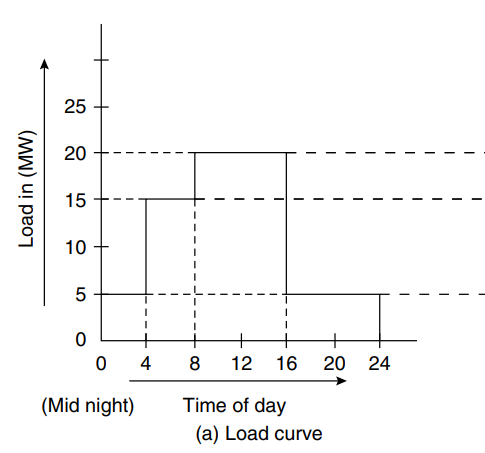
What is a Load Curve? A Load Curve, also known as a chronological load curve, is a graphical representation of the variation of electrical load on a power station over a specific period (typically 24 hours). The curve plots load (in MW) on the Y-axis against time (in hours) on the X-axis. It is useful for identifying peak demand periods and helps in determining the generating capacity required.

Key Features:

• Indicates daily, weekly, monthly, or yearly load patterns.
• Helps in scheduling generation and maintenance.
• Useful in calculating load factor and energy consumption.

Example: Consider a daily load cycle as follows:

From the above data, a chronological load curve can be plotted to show how demand changes throughout the day.

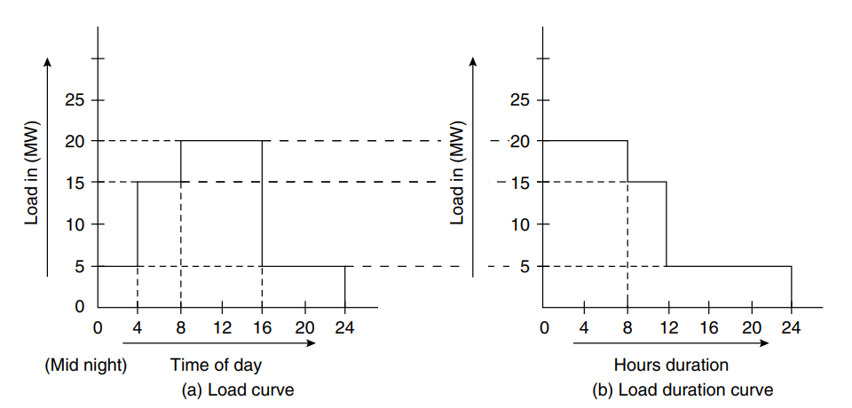
What is a Load Duration Curve? A Load Duration Curve (LDC) is a rearranged version of the load curve where the loads are sorted in descending order, rather than chronologically. This curve shows how long a particular load level is maintained during the observed period.

Key Features:

• X-axis: Time duration (in hours)
• Y-axis: Load (in MW)
• Useful in economic analysis and planning for base load and peaking power plants.

Duration Table Example:

This table is used to construct the load duration curve (Figure b).

Significance of Load and Load Duration Curves

• Operational Planning: Helps in scheduling base load and peak load plants.
• Economic Dispatch: Enables optimal distribution of loads across multiple generation units.
• Cost Efficiency: Influences fixed and variable cost estimations.
• Capacity Planning: Guides decisions on plant sizing and investment.
• Reliability and Maintenance: Aids in maintenance scheduling without affecting supply.

In off-grid regions like rural Kenya, where utility connections are unavailable or unreliable, engineers use Load Duration Curves to design solar-powered microgrids:

1. Data Collection: NGOs collect energy usage patterns like lighting (4 hours), water pumps (2 hours), and refrigeration (24 hours).
2. Load Analysis: These loads are ranked and plotted in an LDC.
3. System Design:
   • Base Load (e.g., refrigeration): handled by solar and batteries.
   • Peak Load (e.g., water pumps): handled by surplus solar or backup sources.
4. Result: Optimised panel and battery size → lower costs, higher reliability, sustainable access.

Conclusion

Understanding Load Curves and Load Duration Curves equips energy professionals with the tools to forecast demand, manage generation efficiently, and design cost-effective power systems. These analytical techniques are foundational in both conventional grid operations and innovative off-grid applications, driving informed decision-making and long-term system reliability.

Want to see how it all works in action?

Watch this video to learn more about load curves and load duration curves.